(NOTE: This turned out to be quite a long post, it might take around an hour to read fully)

Introduction

High school curricula typically introduce basic probability concepts; however, probability theory applied in financial mathematics and statistics requires significantly advanced techniques. To enhance my understanding and proficiency, I will undertake an in-depth exploration of probability theory, encompassing distributions such as Binomial, Gaussian, and Poisson, as well as concepts including random variables, sigma algebras, and probability spaces.

This is by no means a proper text, or learning resource. This is simply what I would've wanted to read, when I was getting started with these topics. Here are the resources I used to learn these topics (still learning, but more or less understood the basics).

Resources

1. MIT OCW 18.S096: youtube link, website link. It's pretty good, but required a lot of previous undergrad knowledge so the learning curve was quite steep. It did however introduce me to the right topics to learn, and I learnt them all individually from different resources.
2. Probability and Stochastics for finance, NPTEL: youtube link, Extremely good, especially since it starts right from the highschool level. This is also where I got the inspiration for the Bertrand Paradox, presented ahead.
3. Quantitative Finance 101, FEBS IIT Bhubaneshwar: youtube link. This made me understand sigma algebras, atleast at a level where I can apply them reasonably. It doesn't really assume zero knowledge, but is pretty in depth.
4. Shreve Stochastic Calculus for Finance II: Continuous-Time Models: link. This book was recommended multiple times, no matter where I looked on the internet. It is in-fact the go-to book for this topic.

Apart from these I've used several other miscellaneous sources, which I won't state here for the sake of brevity.

Prerequisites for Reading

High School Math: A solid foundation in algebra, coordinate geometry, trigonometry, and basic probability (e.g., AP Calculus/Statistics, JEE Advanced, IB Math HL, or A-Level Mathematics).

Set Notation: Comfort with basic set notation (e.g., describing points in a plane or intervals).

Geometric Intuition: Ability to visualize geometric shapes like circles and chords.

Curiosity: An interest in exploring advanced probability concepts, such as sigma algebras and probability spaces, introduced in an accessible way.

No prior knowledge of measure theory or advanced probability is needed—we'll build from intuitive ideas to formal concepts together!

The Paradox

Let's start with a question that seems pretty simple, but is deceptively paradoxical with the math taught in high school.

According to Wikipedia it may be formulated as follows:

"Consider an equilateral triangle that is inscribed in a circle. Suppose a chord of the circle is chosen at random. What is the probability that the chord is longer than a side of the triangle?"

This formulation makes it seem like quite an abstract question,

So we may present it alternatively as:

Consider two concentric circles with A and B with radius R and 2R. Given a chord of the circle B is picked at random, find the probability that this chord intersects, the inner circle A.

This reformulation may model practical scenarios, such as piercing a padded sphere to assess whether it impacts an inner core, though this is merely a contextual preference and does not alter the mathematical problem.

Now typically there are Three methods of tackling this problem.

Method 1: Random Midpoint Method

This is the method that occurred to me, when I tried to solve this problem.

If one plays around with the problem long enough, drawing multiple sketches, we might notice this—

The midpoints of all chords that intersect the inner circle, must lie inside the inner circle.

Since any chord $ AB $ of the outer circle that intersects the inner circle must have its perpendicular distance $ d \leq R $, its midpoint $ M $ (at distance $ d $ from $ O $) must lie within or on the inner circle.

Now one can definitely prove this rigorously (and it is a trivial geometric proof), but for our case, let's just say it is true, visually.

Now if we take only the mid points into consideration, and define a coordinate system with the origin at the centre of $ A , B $, we get a sample space that looks like this—

And if we draw our required event on it, we get—

So for some formal definitions—
$$ \begin{aligned} \Omega &= \{(x,y) \in \mathbb{R}^2 \mid x^2 + y^2 \leq (2R)^2\} \newline \mathbb{E} &= \{(x,y) \in \mathbb{R}^2 \mid x^2 + y^2 \leq R^2\} \end{aligned} $$

Now, to calculate $ P(\mathbb{E}) $ we can simply do—

$$ P(\mathbb{E}) = \frac{\pi(R)^2}{\pi(2R)^2} = \frac{1}{4} $$

So our $ P(\mathbb{E}) $ is —

$$ P(\mathbb{E}) = \boxed{\frac{1}{4}} $$

Method 2: Diameter Method

We may also try a more methodical way—

We first pick a point on the circumference of $ B $, say $ P $, then we draw a diameter passing through the center. Now we may vary this line, by an angle $ \theta $ and get all possible chords that pass through the point $ P $. Similarly we may do this for every point on the circumference of $ B $.

here is what it looks like—

here is the visualization of $ \Omega $ and $ \mathbb{E} $ (NOTE: here X is the distance along the circumference of B)

Why $ \frac{\pi}{6} $?
We can clearly see that a right angled triangle is formed when the chord just touches the inner circle (it is tangent). The hypotenuse is $ 2R $ and the base is $ R $. So we may do $ \cos(\theta) = \frac{R}{2R} $ and then inverse it to get $ \theta = \frac{\pi}{6}$.

Formally— $$ \begin{aligned} \Omega &= \{(X, \theta) \in \mathbb{R}^2 \mid X \in (-2\pi R, 2\pi R), \theta \in (0, \pi/2)\} \newline \mathbb{E} &= \{(X, \theta) \in \mathbb{R}^2 \mid X \in (-2\pi R, 2\pi R), \theta \in (0, \pi/6)\} \end{aligned} $$

Or— $$ \begin{aligned} \Omega &= (-2\pi R, 2\pi R) \times (0, \pi/2) \newline \mathbb{E} &= (-2\pi R, 2\pi R) \times (0, \pi/6) \end{aligned} $$

We can now calculate the probability, like— $$ \begin{aligned} P(\mathbb{E}) &= \frac{4\pi R \cdot (\pi/6)}{4\pi R \cdot (\pi/2)} = \frac{1}{3} \newline P(\mathbb{E}) &= \boxed{\frac{1}{3}} \end{aligned} $$

Method 3: Radius Method

Take a chord passing through the center at an elevation $ \theta $ from the horizontal. Now we may consider all parallel chords to the diameter, at that elevation, their perpedicular distance from the center being $ x $. We get—

and the visualization—

The rest of it is elementary, and $ P(\mathbb{E}) $ comes out to— $$ P(\mathbb{E}) = \boxed{\frac{1}{2}} $$

The Contradiction

So, we have Three answers. This is clearly a contradiction. It means somewhere along the way, our approach with highschool math was flawed. This problem is called the Bertrand Paradox. To correct this we would need an even deeper understanding of probability theory, beyond the typical highschool math.
In reality it is the question that may be misunderstood, the right interpretation is crucial to finding the solution to this paradox. We must realise that the choice of our random chord can impact the probability measure. There are different kinds of random.

Unfortunately, we need the proper "advanced probability theory" to properly discuss the resolution, which is what we'll be exploring in this article. I might write a follow-up post for the resolution as this post is already going to get pretty long. If you really want to know the in-depth reason you can check out the Wikipedia Page
(HINT: the answer, for uniform distributions, is $ \frac{1}{2} $)

Terms and Definitions

Understanding the terms and notation is the most crucial part to understanding probability.

Let's try to intuitively find out what are the terms required to make a reasonable comment on the probability of an event.

What is Probability?

One could call it the likelihood or chance, of a certain event happening. (not to be confused with plausibility)

What information would we need to comment on such a matter? Usually we would need to know what it is, whose outcome we are trying to determine— Is it a coin flip? a horse race? a cricket match?— This is is called the Random Experiment (RE).

Say we want to determine the probability that a grain of sand ends up exactly on top of a treasure chest, on a beach, after being washed away. Obviously we cannot make any reasonably accurate prediction of such an event. Why is that so? It is because we do not know the set of all possible outcomes of our random experiment (RE). So to make an accurate comment on the probability of an event, we must also know the set of all possible outcomes of our RE. This set is called the Sample Space ($ \Omega $)

Sample Space

Now the sample space space could be something like—

$$ \Omega = \{Heads, Tails\} $$

for a coin flip to something like—

$$ \Omega = \{1,2,3,4,5,6 \} $$

for a dice roll.

It may also be something complex like—

$$ \Omega = \{(x,y) \in \mathbb{R}^2 \mid 0 \leq x \leq 1, 0 \leq y \leq 1\} $$

i.e any random point on a unit square. Even more complex —

$$ \Omega = \{(x,y) \in \mathbb{R}^2 \mid 0.25 \leq x^2 + y^2 \leq 1\} $$

i.e any random point on a unit disc, that is atleast 0.5 units away from the center. It could also be visualized as a ring.

Finally, can you guess what this represents —

$$ \Omega = \{(x,y,z) \in \mathbb{R}^3 \mid x^2 + y^2 + z^2 = 1, z \geq 0, \sqrt{x^2 + y^2 + (z-1)^2} \leq 1\} $$

Kind of scary isn't it? ( HINT: it's a sphere, with a special condition.)

This should give an idea as to why we need a formal notation for something so intuitive. As we will see later, the theory builds on this and becomes powerful enough to over-take the intuitive approach.

Sigma Algebra

Typically this is part of measure theory, so we'll only cover what we absolutely need to know.

Again Wikipedia says:

In formal terms, a $\sigma$-algebra on a set $ X $ is a nonempty collection $ \Sigma $ of subsets of $ X $ closed under complement, countable unions, and countable intersections. The ordered pair ( $ X $, $ \Sigma $) is called a measurable space.

Too Complicated, Didn't Understand (TC;DU)

Let's start with the simple problem of trying to have complete knowledge of all events that can possibly occur. How do we find this? simple its just all possible subsets of our sample space $ \Omega $— But can we assign probabilities to all of these events?

In some cases, no, we can't.

To put it simply think of something like this—

we have $ \Omega = [0,1] $, now if we say that we want an event ($ E $) where the length of the interval is 0.5.
How many such subsets do you think there are? infinite. It could be $ [0.2, 0.7] $, $ [0.3, 0.8] $, and so on.

Now whats $ P(E)_{[0.2 , 0.7]} $? Common sense would say its 0.5 (which is correct) since it covers exactly half of the sample space. But this is where intuition breaks down, for example let's try the vitali set—

(NOTE: In hindsight, the exploration coming up wasn't necessary, you may skip it if you like.)

---

Vitali Set (Deep Dive)

Suppose we organize the numbers $(x,y)$ from $[0,1]$ into groups based on a set condition, i.e, $ x - y \in \mathbb{Q} $, the difference must be rational. So we could have $0.7 - 0.2 = 0.5$, in the same group, and $0.8 - 0.3 = 0.5$ in the same group.
This splits $[0,1]$ into a uncountably many groups, for instance, one group might include $0.2, 0.7, 0.2 + 1/3, 0.7 + 1/3,$ and so on, as long as the differences are rational.

Suppose, we pick exactly one number from each group to create a set $ V $, called the Vitali set. The rule is that the numbers we pick must not differ by a rational number, because if they did (like 0.2 and 0.7), they'd be in the same group, and we're only allowed one number per group. So something like $ 0.2 $, and $ 1/\sqrt{2} $ etc. This is tricky because there are uncountably many groups, and we rely on the axiom of choice to ensure we can pick one number from each.

So, we've got our Vitali set $ V $, a collection of numbers, one from each group, where no two numbers differ by a rational. Why does this cause trouble? Let's try to assign it a probability $ P(V) = a $. To check if this works, we shift $ V $ by all rational numbers in $ [0, 1] $, like 0, 0.1, 0.2, 0.3, and so on. For each rational $ q $, the set $ V + q $ (where we add $ q $ to each number in $ V $, wrapping around to stay in $ [0, 1] $) is a shifted copy of $ V $. These shifted sets are disjoint—they don't overlap. Why? If some number appeared in both $ V + q_1 $ and $ V + q_2 $, say $ x + q_1 = y + q_2 $, then $ x - y = q_2 - q_1 $, a rational number, which would mean $ x $ and $ y $ are in the same group, contradicting the fact that $ V $ has only one number per group.

The union of all these shifted sets $ V + q $, over all rational $ q \in [0, 1] $, covers all of $ [0, 1] $. Why? Every number in $ [0, 1] $ belongs to some group, and by shifting $ V $'s representative from each group by all possible rational numbers, we hit every number in every group. Since $ P([0, 1]) = 1 $, the probability of this union should be 1. By our probability rule of countable additivity, the probability of the union is the sum of the probabilities of these disjoint sets:

$$ P\left( \bigcup_{q} (V + q) \right) = \sum_{q} P(V + q) $$

Since shifting by a rational doesn't change the "size" of the set (in a uniform measure), each $ V + q $ should have the same probability as $ V $, so $ P(V + q) = a $. There are countably many rational numbers in $ [0, 1] $, so the sum is:

$$ \sum_{q} P(V + q) = \sum_{q} a $$

Now, we're stuck:

• If $ a > 0 $, the sum $ a + a + \dots $ over countably many terms is infinite, which can't equal 1. That's a contradiction.
• If $ a = 0 $, the sum is 0, which also can't equal 1. Another contradiction.

This shows we can't assign a probability to $ V $ without breaking our probability rules. The Vitali set is non-measurable-it's too strange to fit into our probability framework. This is why we can't assign probabilities to every subset of $ \Omega = [0, 1] $. We need a sigma algebra to limit ourselves to subsets that play nice.

---

A sigma algebra $ \mathcal{F} $ is our curated list of "good" subsets-events we can assign probabilities to consistently. It follows three rules:

1. The whole space is included: $ \Omega \in \mathcal{F} $. We need to say "something happens" with probability 1.
2. Closed under complements: If $ A \in \mathcal{F} $, then $ \Omega \setminus A \in \mathcal{F} $ ($\Omega - A$). If "the number is in $ [0.2, 0.7] $" is an event, "the number is not in $ [0.2, 0.7] $" (i.e., $ [0, 0.2) \cup (0.7, 1] $) is too.
3. Closed under countable unions: If $ A_1, A_2, \dots \in \mathcal{F} $, then $ \bigcup_{i=1}^\infty A_i \in \mathcal{F} $. This lets us combine events like $ [0.1, 0.2] \cup [0.3, 0.4] $.

For $ \Omega = [0, 1] $, a sigma algebra includes nice subsets like intervals, their unions, and complements, but leaves out non-measurable sets like the Vitali set.

But for our intents and purposes, one may think of this as a power set, for simplicity.

The Borel Sigma Algebra

TL:DR It's just a sigma algebra but open intervals.

So, what's a Borel sigma algebra? It's the standard sigma algebra for continuous spaces like $ [0, 1] $, $ \mathbb{R} $, or $ \mathbb{R}^2 $, used in problems like the Bertrand paradox. Think of it as the ultimate collection of measurable subsets that makes probability calculations safe and practical.

The Borel sigma algebra, denoted $ \mathcal{B} $, starts with all open sets in your space. In $ \Omega = [0, 1] $, open sets are intervals like $ (0.2, 0.5) $ (not including endpoints). In $ \mathbb{R}^2 $, they're open disks, rectangles, or shapes with smooth boundaries. The Borel sigma algebra is the smallest sigma algebra that contains all these open sets, built by:

1. Including all open sets.
2. Adding their complements (closed sets, like $ [0.2, 0.5] $).
3. Adding all countable unions and intersections of these sets.

This creates a huge collection of measurable sets (called Borel Sets), including:

• Intervals: $ [0.2, 0.5] $, $ (0, 1) $, or single points like $ {0.42} $.
• Unions of intervals: $ [0.1, 0.3] \cup [0.5, 0.7] $.

Probability Measures and Probability Spaces

Probability Measures

So we laid down most of the formal stuff, now to actually define our Probability measure, we may take a function—

$$ P: \mathcal{F} \to [0,1] $$

From domain = $\mathcal{F}$, to codomain/range = $[0,1]$. Note this assigns probabilities to events in $ \mathcal{F} $(similar to what is covered in highschool), and is different from PMFs and PDFs covered later on. It must satisfy:

1. $P(\Omega) = 1$
2. $P(\phi) = 0$
3. Countable additivity: For a countable collection of disjoint sets, $A_1, A_2, \dots \in \mathcal{F}$, $$ P(\bigcup_{i=1}^\infty A_i) = \Sigma_{i=1}^\infty P(A_i) $$

If all of this seems obvious, good. But in most cases it would be advisable to think of continuous probability as different from discrete probability.

Probability Spaces

So from the terms we defined above, now we can finally define our "world", a probability space. Let's simply package all the relevant stuff into a triple of $(\Omega, \mathcal{F}, P)$.

For example, for a (single) fair coin flip—

$$ \begin{aligned} \Omega &= \{H, T\} \newline \mathcal{F} &= \{\phi, \{H\}, \{T\}, \{H, T\}\} \newline P&(\{H\}) = 0.5 , P({\{T\}}) = 0.5 \end{aligned} $$

Random Variables

So we have a sample space, but doing calculations on it could be quite difficult, especially because we don't really have any set ordering. We typically want something in terms of numbers to do anything practical with it. So we introduce Random Variables (RVs), that solve this problem.

Despite the name, a Random Variable is actually a function—
$$ X: \Omega \to \mathbb{R} $$

It assigns a Real Number ($\mathbb{R}$) to every outcome in the sample space ($\Omega$).
Now obviously we can have two types of random variables.

Discrete Random Variables

It usually takes countable values, for example let's take a dice rolled 3 times. Then—

$$ \Omega = \{(i,j,k): i,j,k \in {1,2,3,4,5,6}\} $$

and suppose our random variable ($X$) is the number of 6s, rolled in the 3 tries—

$$ X: \Omega \to \{0,1,2,3\} $$

and also—

$$ X(\omega \in \Omega) = \text{ number of sixes} $$

More formally—

$$ X((i,j,k)) = \Sigma_{m\in\{i,j,k\}} 1_{\{6\}}(m) $$

where $1_{\{6\}}(m)$ is an indicator function, defined as:

$$ 1_{\{6\}}(m) = \begin{cases} 1 & \text{if } m = 6, \newline 0 & \text{if } m \neq 6 \end{cases} $$

But anyways, there are many ways to define a RV.

Then where is the $\sigma$-algebra ($\mathcal{F}$)? This is the question that confused me for a long time.
Think of it something like this—
In the dice roll example above, if we want the probability of the event that the RV takes the value $X=1$ (i.e $P(X=1)$)
We would want the probability of the event defined by the set— $$ \{\omega \in \Omega: X(\omega) = 1\} $$

This looks some thing like $\{(2,6,4),(4,6,5) \dots\}$. Now this set must belong to $\mathcal{F}$, i.e,
$$ \{\omega \in \Omega: X(\omega) = 1\} \in \mathcal{F} $$

This ensures our event is measurable (refer to the Vitali set above for the counter example). But when applied to most real-world scenarios, one doesn't have to actively check for this statement to be true.

Also note, here the $ X $ maps from $ \Omega $ to a Borel Set, in this case $\{0,1,2,3\}$

Continuous Random Variables

More or less similar to the discrete type, except—

$$ X: \Omega \to \mathbb{R}^n \text{ Where } n \in \mathbb{Z} $$

The rest can be inferred. Maybe try to guess what the RV was in the Bertrand Paradox stated earlier.

Probability distributions

The PMF and the PDF

So, we've defined random variables, which turn outcomes in $\Omega$ into numbers, and we've set up our probability space ($\Omega, \mathcal{F}, P$) to assign probabilities to events. But how do we figure out the likelihood of a random variable taking specific values, like "exactly one 6 in three dice rolls" or "the chord's midpoint in the inner circle"? This is where probability distributions come in—they describe how probabilities are spread across the values of a random variable.

The probability measure $ P $, assigns probabilities to events in $ \mathcal{F} $, but as we've seen before RVs aren't events. So just to compute the probability of the subset of events the RV takes directly (like $P(X=1)$), we introduce tools like the PMF and PDF.

Probability Mass Function (PMF)

For a discrete random variable, which takes countable values (like the number of 6s in three dice rolls), the probability mass function (PMF) gives the probability of each possible value:

$$ P(X = x) $$

Let's revisit our dice example. The sample space is—

$$ \Omega = \{(i,j,k): i,j,k \in {1,2,3,4,5,6}\} $$

And $X((i,j,k)) = \Sigma_{m\in\{i,j,k\}} 1_{\{6\}}(m)$, where $1_{\{6\}}(m)$ is—

$$ 1_{\{6\}}(m) = \begin{cases} 1 & \text{if } m = 6, \newline 0 & \text{if } m \neq 6 \end{cases} $$

Here the PMF tells us probabilities like— $ P(X=1) $, i.e only one 6 is rolled, in three tries. Now for simple stuff like this dice roll, even highschool math will suffice, but just to put it out there, $X$ follows a binomial distribution (Will be covered ahead). So the PMF looks something like—

$$ P(X=k) = \binom{3}{k}\cdot\left(\frac{1}{6}\right)^k\cdot\left(\frac{5}{6}\right)^{3-k} \text{ where } k \in \{0,1,2,3\} $$

Here $k = 1$ gives—

$$ P(X=1) = \binom{3}{1}\cdot\left(\frac{1}{6}\right)^1\cdot\left(\frac{5}{6}\right)^{2} = \frac{75}{216} \approx 0.347 $$

Probability Density Function (PDF)

For a continuous random variable, which takes values in a continuum (like the coordinates of a chord's midpoint in the Bertrand paradox), we can't assign probabilities to specific values because $ P(X = x) = 0 $. So what, do we do? Is it just not possible? Of course not! We take an interval of values, like $ P(a \leq X \leq b) $. This should give us the probability that $ X $ lies in the interval $ [a , b] $, which usually won't be zero (To serve as an abstraction, one can think of this as taking a small section of a line, rather than a point on a line. The point will have no length on the line, which makes defining probabilities for it quite difficult, but the small section has some finite length, however small it may be).

How do we do this though? Simple. We define another function, called the probability density function (PDF) ( $ f(x) $ ). We want this function to be some kind of a "density map" of sorts.

So obviously to find the probability of a specific part we'd do—

$$ P(a \leq X \leq b) = \frac{\int_{a}^{b} f(x)dx}{\int_{-\infty}^{\infty} f(x)dx} $$

But that does not look pretty, especially since $ f(x) $ is not normalized. So we conviniently define $ f(x) $ in such a way that—

$$ \int_{-\infty}^{\infty} f(x)dx = 1 $$

So now we get—

$$ P(a \leq X \leq b) = \int_{a}^{b} f(x)dx $$

Also it must be non-negative for all $x$. i.e $f(x)\geq 0 \forall x$ (try to justify this claim, it's pretty intuitive, but the proof is still quite long and excluded for brevity).

Let's do some examples because abstract definitions like this make no sense.

---

Example 1: Uniform Distribution on an Interval (1D)

Scenario: Suppose you're waiting for a bus that arrives randomly between 0 and 10 minutes from now. Let $X$ be the waiting time in minutes, uniformly distributed over $[0, 10]$.

PDF: Since $X$ is equally likely to take any value in $[0, 10]$, the PDF is constant over that interval. The total area under the PDF must be 1:

$$ f(x) = \frac{1}{10}, \quad 0 \leq x \leq 10 $$

(Outside $[0, 10]$, $f(x) = 0$.) Check: $\int_0^{10} \frac{1}{10} \, dx = \frac{10}{10} = 1$.

Probability: What's the probability you wait between 2 and 5 minutes ($P(2 \leq X \leq 5)$)?

$$ P(2 \leq X \leq 5) = \int_2^5 \frac{1}{10} \, dx = \frac{5 - 2}{10} = \frac{3}{10} = 0.3 $$

Intuition: The PDF is a flat line at height $\frac{1}{10}$. The interval $[2, 5]$ has length 3, so the area is $3 \cdot \frac{1}{10} = 0.3$.

It looks something like—

---

For the sake of brevity, we'll go straight to the named distributions from here, but maybe try to think up a few more examples, before we do. Maybe try to get an exponential distribution (i.e in terms of $e^k \text{ or } a^k$)? (Remember you must normalize them in some way to get $f(x)$)

The Binomial distribution

We've already seen the binomial distribution sneak into our dice example, where we calculated the probability of rolling exactly one 6 in three tries. But what exactly is this distribution, and why is it so important? Let's break it down.

Let's start with the main question:

Given a fixed number of trials (n), flipping a fair coin, calculate the probability of getting exactly 1 heads in these n trials.

Simple high school math right?
But let's visualize it—

Notice that if we select a path all the way down to the bottom, the probabilities of each branch get multiplied. In our case, as it's a fair coin, $ p = (1-p) = 0.5 $. here we only need 1 heads, so we must continue on the rightmost branch, and select the place where we get our heads. We can select the "branch" where we make the split with—

$$ \binom{n}{1} = n $$

And our final probability will look like—

$$ \binom{n}{1}\cdot(0.5)^1\cdot(0.5)^{(n-1)} $$

So to generalize this:
$$ \begin{aligned} p:& \text{ Probability of success.} \newline n:& \text{ Number of trials} \newline k:& \text{ Required number of successes} \end{aligned} $$

So we get a RV, $X$, and— $$ P(X=k) = \binom{n}{k}\cdot(p)^k\cdot(1-p)^{(n-k)} $$ —Is the PMF. Here, $\binom{n}{k}$ counts the ways to choose $k$ successes out of $n$ trials, $p^k$ is the probability of $k$ successes, and $(1 - p)^{n - k}$ covers the failures. Here is the graph ($n=10, p=0.5$)—

The green lines are the floored values of $X$, i.e Integers, where as the red curve is the extension of this binomial distribution. Can you point out what's wrong with it? yeah. The red graph may cause confusion, as the binomial distribution is discrete in nature, so it shouldn't have a continuous graph. So the real binomial distribution is the green lines only, or more accurately, only the points corresponding to integral values of $X$.

By the way, if $X$ follows a Binomial distribution, we say $ X \sim \text{Binomial}(n, p) $, in math language. Now the fun part—

Mean (Expected Value)

We want the expected value, $E[X]$, which is like the average number of successes we'd expect over many, many trials. The probability of getting exactly $k$ successes is given by the binomial probability mass function (PMF):

$$ P(X = k) = \binom{n}{k} \cdot p^k \cdot (1 - p)^{n - k} $$

To find $E[X]$, we weigh each possible number of successes $k$ by its probability:

$$ E[X] = \sum_{k=0}^n k \cdot \binom{n}{k} \cdot p^k \cdot (1 - p)^{n - k} $$

Notice that when $k = 0$, the term is $0 \cdot P(X = 0) = 0$, so it contributes nothing. Let's skip it and start from $k = 1$:

$$ E[X] = \sum_{k=1}^n k \cdot \binom{n}{k} \cdot p^k \cdot (1 - p)^{n - k} $$

Now, that $k \cdot \binom{n}{k}$ looks a bit tricky. Let's play with it. There's a neat identity, taught in highschool, that can be used here:

$$k \cdot \binom{n}{k} = n \cdot \binom{n-1}{k-1}$$

Let's actually use it:

$$ E[X] = \sum_{k=1}^n \left[ n \cdot \binom{n-1}{k-1} \right] \cdot p^k \cdot (1 - p)^{n - k} = n \sum_{k=1}^n \binom{n-1}{k-1} \cdot p^k \cdot (1 - p)^{n - k} $$

To make this sum friendlier, let's shift the index. Set $j = k - 1$. When $k = 1$, $j = 0$; when $k = n$, $j = n-1$. Also, adjust the exponents: $p^k = p^{j+1} = p \cdot p^j$ and $(1 - p)^{n - k} = (1 - p)^{(n-1) - j}$. So the sum becomes:

$$ E[X] = n \sum_{j=0}^{n-1} \binom{n-1}{j} \cdot (p \cdot p^j) \cdot (1 - p)^{(n-1) - j} = n p \sum_{j=0}^{n-1} \binom{n-1}{j} \cdot p^j \cdot (1 - p)^{(n-1) - j} $$

That sum looks familiar—it's the total probability of a binomial random variable with $n-1$ trials and probability $p$, which sums to 1 (since it's the sum of all probabilities for a $\text{Binomial}(n-1, p)$ distribution). So:

$$ \sum_{j=0}^{n-1} \binom{n-1}{j} \cdot p^j \cdot (1 - p)^{(n-1) - j} = 1 $$

Thus:

$$ E[X] = n p \cdot 1 = n p $$

$$ \boxed{E[X] = n p} $$

That looks like something we'd expect, right? If you flip a coin $n$ times with success probability $p$, you expect $n p$ successes on average. Like, if you flip a fair coin ($p = 0.5$) 10 times, you'd expect about 5 heads.

Variance

Now for the variance, $\text{Var}(X) = E[X^2] - (E[X])^2$, which tells us how spread out our number of successes is. Calculating $E[X^2]$ directly is a bit messy, so let's be clever and compute $E[X(X-1)]$ first, which is like looking at pairs of successes. Then we'll relate it to $E[X^2]$. Start with:

$$ E[X(X-1)] = \sum_{k=0}^n k (k-1) \cdot \binom{n}{k} \cdot p^k \cdot (1 - p)^{n - k} $$

When $k = 0$ or $k = 1$, $k(k-1) = 0$, so those terms vanish. Start at $k = 2$:

$$ E[X(X-1)] = \sum_{k=2}^n k (k-1) \cdot \binom{n}{k} \cdot p^k \cdot (1 - p)^{n - k} $$

Another cool identity: $k (k-1) \cdot \binom{n}{k} = n (n-1) \cdot \binom{n-2}{k-2}$. (Just kidding, its the same thing applied twice) $$ \begin{aligned} E[X(X-1)] =& \sum_{k=2}^n \left[ n (n-1) \cdot \binom{n-2}{k-2} \right] \cdot p^k \cdot (1 - p)^{n - k} \newline
=& n (n-1) \sum_{k=2}^n \binom{n-2}{k-2} \cdot p^k \cdot (1 - p)^{n - k} \end{aligned} $$

Reindex with $j = k - 2$. When $k = 2$, $j = 0$; when $k = n$, $j = n-2$. Exponents adjust: $p^k = p^{j+2} = p^2 \cdot p^j$, and $(1 - p)^{n - k} = (1 - p)^{(n-2) - j}$. So:

$$ E[X(X-1)] = n (n-1) p^2 \sum_{j=0}^{n-2} \binom{n-2}{j} \cdot p^j \cdot (1 - p)^{(n-2) - j} $$

That sum is the total probability for a $\text{Binomial}(n-2, p)$, which equals 1:

$$ E[X(X-1)] = n (n-1) p^2 \cdot 1 = n (n-1) p^2 $$

Now, relate $E[X(X-1)]$ to $E[X^2]$:

$$ E[X(X-1)] = E[X^2 - X] = E[X^2] - E[X] $$

So:

$$ E[X^2] = E[X(X-1)] + E[X] = n (n-1) p^2 + n p $$

Now compute the variance:

$$ \text{Var}(X) = E[X^2] - (E[X])^2 = \left[ n (n-1) p^2 + n p \right] - (n p)^2 $$

Simplify:

$$ = n (n-1) p^2 + n p - n^2 p^2 = n^2 p^2 - n p^2 + n p - n^2 p^2 = n p - n p^2 = n p (1 - p) $$

$$ \boxed{\text{Var}(X) = n p (1 - p)} $$

Interesting! The variance $n p (1 - p)$ is highest when $p = 0.5$, meaning the outcome is most uncertain when success and failure are equally likely. For $p$ close to 0 or 1, the variance shrinks, as the outcome is more predictable.

So, our final answers are:

$$ \begin{aligned} E[X] &= \boxed{n p} \newline \text{Var}(X) &= \boxed{n p (1 - p)} \end{aligned} $$

The Poisson distribution

Imagine we're running a website, and we're interested in the number of visitors arriving in a given hour, and possibly predict average traffic and future probabilities of extreme traffic with it. (for e.g how likely 10k visitors are, etc)
How do we model this, with the math we've learnt? How about we make every second a RV ($X$)? We'd have two possibilities:

1. A user visits the site (success)
2. No one visits the site (failure)

Looks familiar? That's because $X$ follows a binomial distribution! But clearly anyone can see the limitations here—

1. What if two users visit in 1 second.
2. Computationally infeasible. (we're evaluating the binomial formula. every. single. second. i.e 3600 times an hour, or even higher for finer precision)
3. $P(\text{success})$ is tiny.

Deriving the Poisson from the Binomial

So instead, how about we calculate the average rate of visitors (the mean), say $\lambda$, and try to do something with that—
But what exactly? We mainly want to model the probability of getting $k$ (5 or 10 or 20) visitors an hour, simply from the fact that we know that on average there are $\lambda$ visitors an hour. Let's start with the binomial version—

$$ P_{\text{binomial}}(X=k) = \binom{n}{k}\cdot(p)^{k}\cdot(1-p)^{n-k} $$

But now our no. of trials $n \to \infty$ , and our probability of success $p \to 0$. With limits, that'd look something like—

$$ P_{\text{poisson}}(X=k) = \lim_{n \to \infty ;\text{ } p \to 0} \binom{n}{k}\cdot(p)^{k}\cdot(1-p)^{n-k} $$

Now even writing it out looks, funky, so we must find a way to reduce this to one variable. Recall that the mean of a binomial was $np$. But we set the average rate of visitors to $\lambda$, so—

$$ \begin{aligned} np &= \lambda \newline p &= \frac{\lambda}{n} \end{aligned} $$

Now let's put this back in that limit, so—

$$ P_{\text{poisson}}(X=k) = \lim_{n \to \infty} \binom{n}{k}\cdot\left(\frac{\lambda}{n}\right)^{k}\cdot\left(1-\frac{\lambda}{n}\right)^{n-k} $$

Looks a bit easier now... Oh, let's expand the combination to it's factorial notation—

$$ P_{\text{poisson}}(X=k) = \lim_{n \to \infty} \left(\frac{n!}{k!(n-k)!} \right) \cdot \left(\frac{\lambda}{n}\right)^{k} \cdot \left(1-\frac{\lambda}{n}\right)^{n-k} $$

So we have three terms we have to deal with—

$$ \begin{aligned} \lim_{n \to \infty} &\left(\frac{n!}{k!(n-k)!} \right) \newline \lim_{n \to \infty} &\left(\frac{\lambda}{n}\right)^{k} \newline \lim_{n \to \infty} &\left(1-\frac{\lambda}{n}\right)^{n-k} \end{aligned} $$

Expand the first one—

$$ \lim_{n \to \infty} \left(\frac{n(n-1)(n-2) \dots (n-k+1)\cdot(n-k)(n-k-1)\dots}{k!(n-k)(n-k-1)\dots} \right) $$

Notice how everything after the dot gets cancelled with the denominator? But also notice, that $n \to \infty$, so $n \approx (n-1) \approx (n-k+1)$. Yes, there is a proper mathematical way to do it, but let's just keep it intuitive and move on. So now our expression is—

$$ \lim_{n \to \infty} \left(\frac{n^k}{k!} \right) $$

Do you see it? Let's bring back the second part—

$$ \lim_{n \to \infty} \left(\frac{n^k}{k!} \right)\cdot \left(\frac{\lambda}{n}\right)^{k} $$

It gets cancelled! So together we're only left with normal variables for the first and second part, i.e — $$ \lim_{n \to \infty} \left(\frac{\lambda^k}{k!} \right) $$

For the last part, we have to get a little creative (although it's a simple trick taught in JEE prep. and stuff). Let $L$ be the limit for the 3rd part.

$$ L = \lim_{n \to \infty} \left(1-\frac{\lambda}{n}\right)^{n-k} $$

Taking natural log on both sides we get—

$$ \ln(L) = \lim_{n \to \infty} (n-k)\ln\left(1-\frac{\lambda}{n}\right) $$

Of course, there are a few nuances to this step, but let's not bother. Rewriting it to get $0/0$ form—

$$ \ln(L) = \lim_{n \to \infty} \frac{\ln\left(1-\frac{\lambda}{n}\right)}{\frac{1}{(n-k)}} $$

What do we do next? L'Hopital of course, because we're lazy—

$$ \ln(L) = \lim_{n \to \infty} \frac{\frac{1}{1-\frac{\lambda}{n}}\cdot\frac{\lambda}{n^2}}{\frac{-1}{(n-k)^2}} $$

Hm— $(n-k)^2 \approx n^2$ so let's just cancel them, and put $\lambda / n = 0$. And with that we've got rid of the limit—

$$ \ln(L) = -\lambda $$

So— $$ L = e^{-\lambda} $$

Put it all back together— $$ \boxed{P_{\text{poisson}}(X=k) = \frac{\lambda^k \cdot e^{-\lambda}}{k!}} $$

Where, $X \sim \text{Poisson}(\lambda) $

And here is the graph($\lambda = 2$) —

Of course the red graph is wrong, and the green one is the true graph (floored). Notice something peculiar? Getting $\lambda - 1$ has the same probability as getting $ \lambda $ visitors (when $\lambda$ is an integer, which it always is in our case).

Mean (Expected Value) & Variance

To save time, I'll just say it (Feel free to derive it on your own, it's not that hard). The mean and variance are—

$$ \begin{aligned} E[X] &= \lambda \newline \text{Var}(X) &= \lambda \end{aligned} $$

The mean is understandable because that's what we assumed, but why does the variance depend on the mean?
What does our expected value, have to do with spread? Think about it.

The Gaussian (Normal) distribution

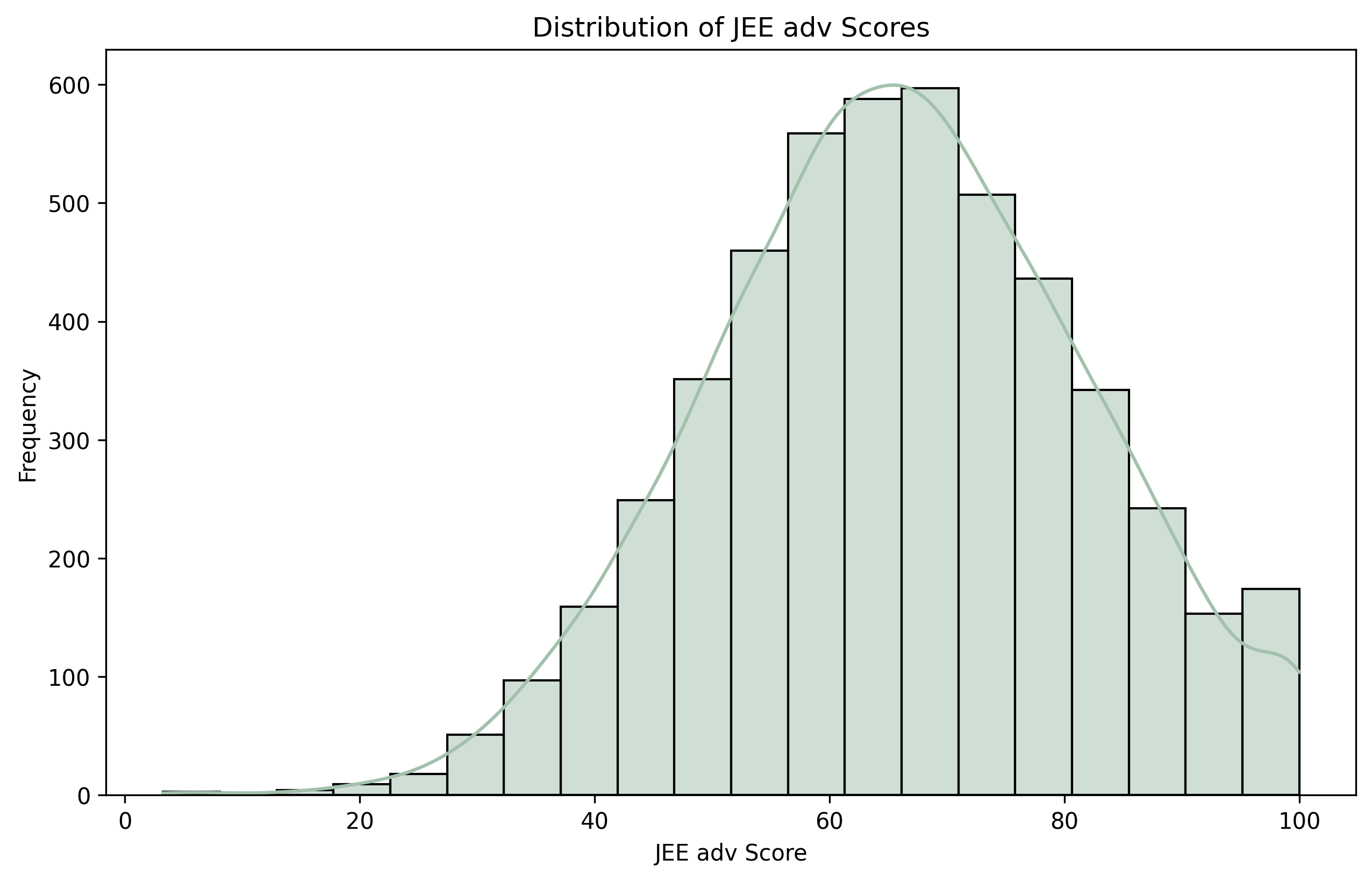
Take a look at this mark distribution for JEE:

Or this marathon finish-time distribution—

Or stock prices (random walk) over a long time—

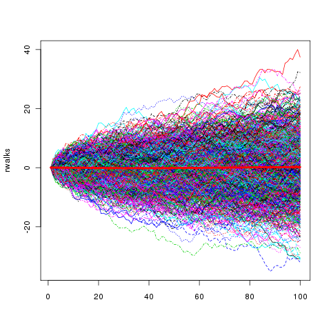
Did you spot it? exactly all of them look kind of "bell-shaped". That's called a normal/gaussian distribution—
But what exactly is the question it is trying to answer? It tries to answer this question:

What's the likelihood that a continuous random variable, shaped by many small, independent random effects, falls within a specific range?

This applies to scenarios like test scores, where individual strengths and weaknesses average out, or stock prices, where daily fluctuations accumulate. Unlike the binomial (discrete trials) or Poisson (rare events), the Gaussian handles continuous data with a characteristic bell shape, which turns out to be pretty useful in real-world applications, beyond just recreational mathematics.

Deriving the Gaussian from the Binomial

(NOTE: Heavy math incoming, it scares me too. It's better to derive it by yourself, which also makes it easier to understand. When starting out, it's better to just memorize the formula and learn to apply it before getting into this derivation, as it involves a lot of complicated approximations)

The binomial distribution models the number of successes in $n$ trials, each with success probability $p$. Suppose we're flipping a fair coin ($p = 0.5$) many times, say $n = 1000$, and we want the probability of getting $k$ heads. The PMF is:

$$ P(X = k) = \binom{n}{k} p^k (1 - p)^{n - k} $$

For large $n$, computing $\binom{n}{k}$ directly is a nightmare. Plus, the distribution starts to look smooth, almost like a continuous curve (remember the green lines in the binomial graph?). Let's explore what happens when $n \to \infty$.

(NOTE: Unlike the poisson distribution, here $p$ does not tend to 0)

First, let's "center" the distribution. The mean of a binomial is $E[X] = n p$, and the variance is $\text{Var}(X) = n p (1 - p)$. For $p = 0.5$, the mean is $n/2$, and the standard deviation is $\sqrt{n \cdot 0.5 \cdot 0.5} = \sqrt{n/4} = \sqrt{n}/2$. Let's standardize the random variable $X$ to see its behavior:

$$ Z = \frac{X - n p}{\sqrt{n p (1 - p)}} $$

Wait, what exactly did we do? why "standardize" it?
Remember how we normalized continuous RVs? exactly. We'd prefer a more standardized way to represent the same distribution, which would make it easier to compare to other such distributions. So we ask it: "How far is $ X $ from its average, relative to its typical spread?".

Here, $Z$ measures how many standard deviations $X$ is from the mean, which answers the first question.

Now, We want the probability density of $Z$ as $n$ grows large. To do this, let's approximate $P(X = k)$ for large $n$ using Stirling's approximation, which simplifies factorials:

$$ n! \approx \sqrt{2 \pi n} \left( \frac{n}{e} \right)^n $$

For the binomial coefficient:

$$ \binom{n}{k} = \frac{n!}{k! (n - k)!} \approx \frac{\sqrt{2 \pi n} \left( \frac{n}{e} \right)^n}{\sqrt{2 \pi k} \left( \frac{k}{e} \right)^k \sqrt{2 \pi (n - k)} \left( \frac{n - k}{e} \right)^{n - k}} $$

Simplify:

$$ \binom{n}{k} \approx \frac{\sqrt{2 \pi n}}{\sqrt{2 \pi k} \sqrt{2 \pi (n - k)}} \cdot \frac{\frac{n^n}{e^n}}{\frac{k^k (n - k)^{n - k}}{e^k e^{n - k}}} = \sqrt{\frac{n}{2 \pi k (n - k)}} \cdot \frac{n^n}{k^k (n - k)^{n - k}} $$

Now, the binomial PMF is:

$$ P(X = k) = \binom{n}{k} p^k (1 - p)^{n - k} \approx \sqrt{\frac{n}{2 \pi k (n - k)}} \cdot \frac{n^n}{k^k (n - k)^{n - k}} \cdot p^k (1 - p)^{n - k} $$

Let's express $k$ around the mean: set $k = n p + x \sqrt{n p (1 - p)}$, so $x$ represents deviations in standard deviation units (like $Z$). Then:

$$ n - k = n - (n p + x \sqrt{n p (1 - p)}) = n (1 - p) - x \sqrt{n p (1 - p)} $$

For large $n$, assume $k \approx n p$, so $k (n - k) \approx (n p) (n (1 - p)) = n^2 p (1 - p)$. The square root term becomes:

$$ \sqrt{\frac{n}{2 \pi k (n - k)}} \approx \sqrt{\frac{n}{2 \pi n^2 p (1 - p)}} = \frac{1}{\sqrt{2 \pi n p (1 - p)}} $$

Now tackle the rest. The term $\frac{n^n}{k^k (n - k)^{n - k}} p^k (1 - p)^{n - k}$ needs careful handling. Take its logarithm to simplify:

$$ \ln \left( \frac{n^n p^k (1 - p)^{n - k}}{k^k (n - k)^{n - k}} \right) = n \ln n + k \ln p + (n - k) \ln (1 - p) - k \ln k - (n - k) \ln (n - k) $$

(NOTE: After this, writing out the rest of it will simply look messy. So it's better to do it by oneself.)

Substitute $k = n p + x \sqrt{n p (1 - p)}$ and use Taylor expansions around the mean. This gets messy, so let's focus on the exponent. For large $n$, the binomial PMF approximates a density. After substituting and simplifying (using normal approximation techniques), we get:

$$ \boxed{P(X = k) \approx \frac{1}{\sqrt{2 \pi n p (1 - p)}} e^{-\frac{(k - n p)^2}{2 n p (1 - p)}}} $$

For the standardized variable $Z$, the density of $Z \approx x$ is:

$$ f(z) = \frac{1}{\sqrt{2 \pi}} e^{-\frac{z^2}{2}} $$

This is the standard normal distribution, $Z \sim \mathcal{N}(0, 1)$, with mean 0 and variance 1. For a general normal distribution $X \sim \mathcal{N}(\mu, \sigma^2)$, where $\mu$ is the mean and $\sigma^2$ is the variance, we transform $Z = \frac{X - \mu}{\sigma}$, so the PDF of $X$ is:

$$ \boxed{f(x) = \frac{1}{\sqrt{2 \pi \sigma^2}} e^{-\frac{(x - \mu)^2}{2 \sigma^2}}} $$

Let's verify it integrates to 1:

$$ \int_{-\infty}^{\infty} \frac{1}{\sqrt{2 \pi \sigma^2}} e^{-\frac{(x - \mu)^2}{2 \sigma^2}} dx $$

Substitute $u = \frac{x - \mu}{\sigma}$, so $x = \mu + \sigma u$, $dx = \sigma du$:

$$ \int_{-\infty}^{\infty} \frac{1}{\sqrt{2 \pi \sigma^2}} e^{-\frac{u^2}{2}} \sigma du = \frac{1}{\sqrt{2 \pi}} \int_{-\infty}^{\infty} e^{-\frac{u^2}{2}} du = 1 $$

(The integral equals $\sqrt{2 \pi}$, so it normalizes correctly.) The PDF is non-negative, satisfying all requirements.

Here's the graph for $\mathcal{N}(0, 1)$:

Mean and Variance

The mean of $X \sim \mathcal{N}(\mu, \sigma^2)$ is:

$$ E[X] = \int_{-\infty}^{\infty} x \cdot \frac{1}{\sqrt{2 \pi \sigma^2}} e^{-\frac{(x - \mu)^2}{2 \sigma^2}} dx $$

Substitute $u = \frac{x - \mu}{\sigma}$, so $x = \mu + \sigma u$, $dx = \sigma du$:

$$ E[X] = \int_{-\infty}^{\infty} (\mu + \sigma u) \cdot \frac{1}{\sqrt{2 \pi}} e^{-\frac{u^2}{2}} du = \mu \int_{-\infty}^{\infty} \frac{1}{\sqrt{2 \pi}} e^{-\frac{u^2}{2}} du + \sigma \int_{-\infty}^{\infty} u \cdot \frac{1}{\sqrt{2 \pi}} e^{-\frac{u^2}{2}} du $$

The first integral is 1 (total probability). The second is 0 (since $u e^{-\frac{u^2}{2}}$ is odd). So:

$$ E[X] = \mu $$

For variance, compute $E[(X - \mu)^2]$:

$$ \text{Var}(X) = \int_{-\infty}^{\infty} (x - \mu)^2 \cdot \frac{1}{\sqrt{2 \pi \sigma^2}} e^{-\frac{(x - \mu)^2}{2 \sigma^2}} dx $$

Using $u = \frac{x - \mu}{\sigma}$:

$$ \text{Var}(X) = \int_{-\infty}^{\infty} (\sigma u)^2 \cdot \frac{1}{\sqrt{2 \pi}} e^{-\frac{u^2}{2}} du = \sigma^2 \int_{-\infty}^{\infty} u^2 \cdot \frac{1}{\sqrt{2 \pi}} e^{-\frac{u^2}{2}} du $$

The integral is the variance of a standard normal, which is 1 (by definition or computation). Thus:

$$ \text{Var}(X) = \sigma^2 $$

So:

$$ \begin{aligned} E[X] &= \boxed{\mu} \newline \text{Var}(X) &= \boxed{\sigma^2} \end{aligned} $$

Conclusion

Recap

This blog is not a formal learning resource but a personal account of my journey exploring advanced probability as a high school student, not a professional. It extends beyond high school basics into concepts essential for financial mathematics and statistics. The Bertrand Paradox illustrates the challenges of defining randomness, producing conflicting probabilities ($ 1/4 $, $ 1/3 $, $ 1/2 $) for a chord's length depending on the selection method, highlighting the need for a rigorous framework. This post does not resolve the paradox due to its length, but the concepts introduced provide tools to tackle it, with a follow-up post planned for the future.

Key concepts covered include:

• Sample Space ($ \Omega $): The set of all possible outcomes of a random experiment.
• Sigma Algebra ($ \mathcal{F} $): A collection of measurable subsets of $ \Omega $, closed under complement and countable unions, ensuring consistent probability assignments (e.g., excluding non-measurable Vitali sets).
• Probability Measure ($ P $): A function that maps events in $ \mathcal{F} $ to $[0,1]$, satisfying $ P(\Omega) = 1 $ and countable additivity.
• Probability Space ($ (\Omega, \mathcal{F}, P) $): The triple defining the sequence.

• Random Variables: Functions $ X: \Omega \to \mathbb{R} $, either discrete (countable values) or continuous (continuum values), with probabilities assigned to events in $ \mathcal{F} $.

• Probability Distributions:

  1. Binomial Distribution: Models $ k $ successes in $ n $ trials, with PMF
     $$ \begin{aligned} P(X = k) &= \binom{n}{k} p^k (1-p)^{n-k},\newline \text{mean } E[X] &= np,\newline \quad \text{variance } \text{Var}(X) &= np(1-p). \end{aligned} $$
  2. Poisson Distribution: Approximates binomial for large $ n $ and small $ p $, with PMF
     $$ P(X = k) = \frac{\lambda^k e^{-\lambda}}{k!}, \newline \text{mean and variance both } \lambda. $$
  3. Gaussian Distribution: Describes continuous variables from cumulative small effects, with PDF
     $$ f(x) = \frac{1}{\sqrt{2\pi \sigma^2}} e^{-\frac{(x-\mu)^2}{2 \sigma^2}}, \newline \text{mean } \mu, \quad \text{variance } \sigma^2. $$

Drawing on resources like MIT OCW, NPTEL, and Shreve's Stochastic Calculus, this exploration establishes a foundation for addressing complex problems in quantitative finance, equipping readers to approach problems like those in the Bertrand Paradox with structured probabilistic concepts.

Personal Remarks

I never expected this post to take so long. I encountered numerous challenges while trying to convey what I wanted to say— although this isn't my first time typing out latex code, it was still quite a hassle. There were also various other unforeseen hinderances, that slowed this down even more. Originally I intended this post to simply be a weekend thing— but it just didn't seem to end. It has been nearly a month since the due date. (Check the Github commit history, if want to know what I'm talking about: Github commit history)
In the end I had to cut out the applications, as well as the intuitive exploration of the Gaussian, which I was very much looking forward to share. However due the length of this post, as well as the time it has taken, I simply cannot continue it any further. I might post higher-level posts exploring actual quantitative trading stuff, but this series has to be put on hold for a while.

The resources I recommended however, are leagues better than this post, and worth exploring, if one has the time. I hope this post might've inspired atleast one person to dive into this world, and experience the true beauty of math, that they try to hide from us in High School.